Seismology has provided fundamental data on the Earth’s inner structure. Thanks to the recordings of earthquake vibrations (the seismographs) scientist were able to indirectly look inside our planet, rather like doing the Earth a CT scan.
An earthquake is a natural phenomenon which occurs when tensions in the crust abruptly break their balance in unstable areas. When those tensions grow higher than the rocks’ ability to resist them, fractures and slippages take place. At the same time, elastic waves are generated in the rupture point. They are both transverse and longitudinal waves with respect to the direction of propagation, which occurs through the whole planet.
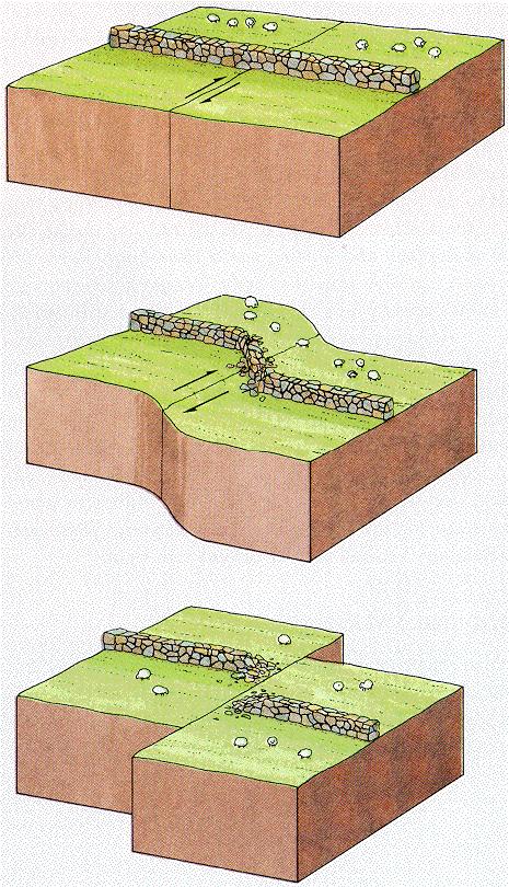
Reid’s elastic rebound
While examining the surface displacements occurred after the San Francisco earthquake of 1906, Henry Fielding Reid, (1859 – 1944), professor of geology at the Johns Hopkins University, came to the conclusion that the earthquake must have caused an “elastic rebound” of the accumulated stress.

Henry Fielding Reid, (1859 – 1944)
If a piece of rubber is broken or cut, the elastic energy stored during deformation will be released at once. In the same way, Earth’s crust can gradually store elastic stress to be suddenly released during an earthquake. This gradual accumulation and sudden release after deformation is called the “elastic rebound theory” of earthquakes (top).
Seismic waves
Two types of elastic waves can propagate in a solid body independently: “longitudinal waves” and “transverse waves”.
The former propagate as alternating compressions and dilatations. As transverse waves propagate, vibrations occur on perpendicular planes to the direction of propagation. Longitudinal waves are faster and reach the measuring instruments earlier, being recorded as P waves (pressure waves, “a” in the picture below).
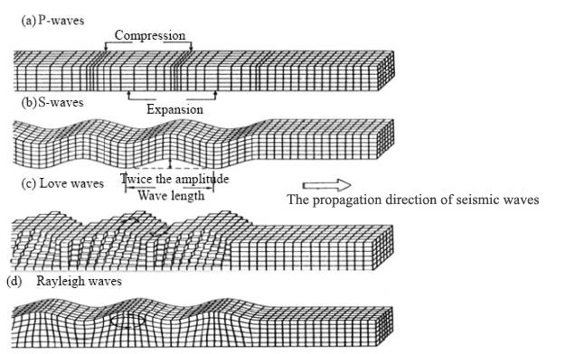
After a while, transverse waves are also recorded as S waves (shear waves, “b” above). A third group of waves should concern us more, since they travel only along the Earth’s surface: the L waves (long waves). Rayleigh’s waves (“d” in the picture above) are similar to those formed when throwing a stone in the water. They cause the terrain to vibrate along retrograde elliptical orbits with respect to the direction of propagation. Love’s waves (“c”) cause the terrain to vibrate along the horizontal plane. The movement of the points the waves pass through is transverse and horizontal with respect to the direction of propagation.
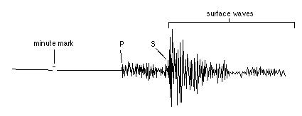
Different arrival times for P and S waves
Seismic waves generating from an earthquake’s hypocenter are therefore of two kinds: compression and shear waves. The faster P waves are the first impulse on a seismograph; the slower S waves cannot be generated, nor they propagate in fluids. The delay between the arrival times of P and S waves at a recording station is therefore a function of the distance of the station from the epicenter. Putting together seismographs of the same earthquake from different stations we obtain curves called dromochrones, which connect the P and S waves arrival times on the diagram (below).
Dromochrone for P and S waves
With a simple graphing procedure it is possible to locate the epicenter area of an earthquake by knowing its distance from at least three different recording stations. Three circles centered on the stations, with a radius equal to the station’s distance from the epicenter (calculated from the P and S waves arrival times), will overlay at the epicenter area (below).
Triangulation among at least three seismometers allows locating the epicenter area
The energy released by an earthquake (Newton x meter) is today expressed as seismic moment M0, obtained by multiplying the fractured area times the average displacement along the fault times the rigidity of the involved rocks (the shear modulus representing the stress/strain ratio at the fault). It is generated by computer calculations on the seismographs and it is a measure of the energy released by earthquakes according to the moment magnitude scale (MMS).
Charles Francis Richter (1900 – 1985), American seismologist at Caltech, is the father of modern magnitude scales used to “measure” earthquakes. In 1935, after suggestion from his colleague Beno Gutenberg of the same university, he used a logarithmic scale in the attempt to relate the seismographs’ wave amplitudes to the distance from the epicenter (an idea inspired by an article by the Japanese seismologist Kiyoo Wadati).

Charles Francis Richter (1900 – 1985)
He soon realized how comfortable it was to use the amplitudes’ base 10 logarithm for graphing the values (the diagram’s dimensions would have grown too large otherwise). In developing his famous Richter scale, he chose the measuring unit as the earthquake that caused a 1 mm maximum displacement on a particular type of seismographer at a 100 km distance from the epicenter. This would have defined Magnitude = 0 (Log10 1 = 0), a word he borrowed from his passion for astronomy, where it represents the brightness of stars. The nomograph below can be used to manually calculate the Richter Magnitude ML (local Magnitude) from the maximum amplitude measured on the seismograph and the epicenter distance.
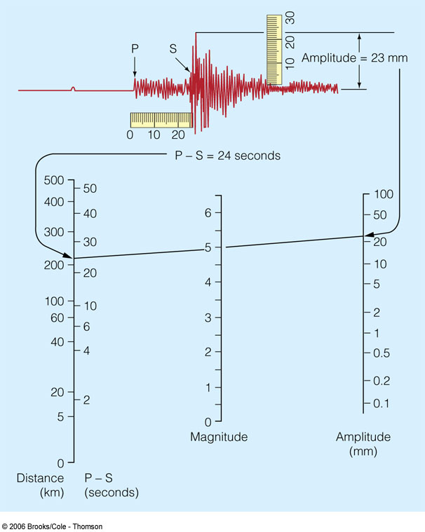
Nomogram for calculating the Richter magnitude from the seismogram: for an S wave amplitude of 23 mm and a 24 seconds arrival time difference we have an ML=5 local Richter magnitude
Since the Richter Scale is a logarithmic one, any value increment in the scale corresponds to an increment of 10 in measured earthquake amplitude (any magnitude increase of one unit is 31.6 times bigger in terms of energy). Today the MMS is the most used, especially for larger earthquakes. In other cases, updated versions of the Richter scale are used.
The most widely used scale today is the MMS (Moment Magnitude Scale), especially for earthquakes larger than ML = 4. Developed in 1979 by seismologist Hiroo Kanamori of Caltech along with Thomas C. Hanks of the USGS, the moment magnitude scale is based on the seismic moment M0 = μDA, a quantity equal to the product of the rock’s rigidity modulus μ, times the mean displacement D along the fault, times the area A of the fault’s portion that moved. Kanamori identified a relationship between seismic moment and energy released by an earthquake and defined a moment magnitude Mw (W = work, work) in a formula that he refined with Hanks:
Mw = 2/3 log10 (M0) – 10.7
where M0 is the seismic moment and the constants were added to make the MMS scale consistent with previous Richter scales.
Intensity scales such as the Mercalli Scale are used to describe the effects caused by an earthquake, which depend on local conditions. An earthquake of a certain magnitude may have different consequences if it takes place in a desert or in a town.

Giuseppe Mercalli, (1850 – 1914)
Giuseppe Mercalli, (1850 – 1914), Italian abbot and seismologist, first created a 10 degree scale that was later upgraded by the Italian physicist Adolfo Cancani and the German geophysicist August Seiberg to become the Mercalli-Cancani-Sieberg (MCS) scale. Richter himself finally modified it in the current Modified Mercalli (MM) 12 degree scale.
Richter and Mercalli scales compared
| Magnitude | Description | Mercalli intensity | Average earthquake effects | Average frequency of occurrence (estimated) |
| Less than 2.0 | Micro | I | Microearthquakes, not felt, or felt rarely by sensitive people. Recorded by seismographs. | Continual/several million per year |
| 2.0–2.9 | Minor | I to II | Felt slightly by some people. No damage to buildings. | Over one million per year |
| 3.0–3.9 | II to IV | Often felt by people, but very rarely causes damage. Shaking of indoor objects can be noticeable. | Over 100,000 per year | |
| 4.0–4.9 | Light | IV to VI | Noticeable shaking of indoor objects and rattling noises. Felt by most people in the affected area. Slightly felt outside. Generally causes none to minimal damage. Moderate to significant damage very unlikely. Some objects may fall off shelves or be knocked over. | 10,000 to 15,000 per year |
| 5.0–5.9 | Moderate | VI to VIII | Can cause damage of varying severity to poorly constructed buildings. At most, none to slight damage to all other buildings. Felt by everyone. Casualties range from none to a few. | 1,000 to 1,500 per year |
| 6.0–6.9 | Strong | VII to X | Damage to a moderate number of well built structures in populated areas. Earthquake-resistant structures survive with slight to moderate damage. Poorly-designed structures receive moderate to severe damage. Felt in wider areas; up to hundreds of miles/kilometers from the epicenter. Strong to violent shaking in epicentral area. Death toll ranges from none to 25,000. | 100 to 150 per year |
| 7.0–7.9 | Major | VIII or greater | Causes damage to most buildings, some to partially or completely collapse or receive severe damage. Well-designed structures are likely to receive damage. Felt across great distances with major damage mostly limited to 250 km from epicenter. Death toll ranges from none to 250,000. | 10 to 20 per year |
| 8.0–8.9 | Great | Major damage to buildings, structures likely to be destroyed. Will cause moderate to heavy damage to sturdy or earthquake-resistant buildings. Damaging in large areas. Felt in extremely large regions. Death toll ranges from 1,000 to 1 million. | One per year | |
| 9.0 and greater | Near or at total destruction – severe damage or collapse to all buildings. Heavy damage and shaking extends to distant locations. Permanent changes in ground topography. Death toll usually over 50,000. | One per 10 to 50 years |